Tracking the precise dropoff location of a delivery in your building.
Tl;DR
I built a time-series classification model that could classify whether or not a person was indoors or outdoors based on the data collected by the 9-DoF sensor on their phone because I was excited to apply to a senior machine learning engineer role at Doorstep.ai. Unfortunately, the company emphasized Leetcode and I did not pass the coding round because i couldn’t code up a solution to a palindrome substring problem. I wrote this project in the span of 3 days over the weekend. The deployable model and steps to replicate the training of the model are here.
You can just do things with time-series data
It is no secret that I love time-series datastreams and I think humanity should get really good at reading, understanding, leveraging, and making predictions from time-series data.
I’ve gleaned some insights while using time-series datasets over the years. Here’s a few:
Learn how to sleep better
When I worked on a project with Fulcra Dynamics I leveraged HealthKit data and other raw data from a continuous glucose monitor. I assembled data at a per second interval and cleansed over 6 months of collection data to produce a multi-modal machine learning approach to find that a patient could get one extra hour of sleep if they just ate their last meal 2-3 hours earlier than they normally did. Intriguingly this is very consistent with the work of Jürgen Aschoff who found that the body’s circadian rhythm is regulated by multiple cues, including the timing of meals.
This dataset was incredibly rich and clean from biased actions because the data was passively collected and required no human intervention. Sure, you could knock the collection accuracy and the precision of the data relative to the human event but that’s an improving trend over time as electronics become more sensitive and the data collection becomes more precise.
Have a job that can’t be stolen by AI
Its no secret that time-series models are incredibly dense matricies. In a typical time-series tensor you’ve got three dimensions:
import numpy as np

tensor = np.array([
    [
        [1, 2, 3],
        [4, 5, 6],
    ],
    [
        [7, 8, 9],
        [10, 11, 12],
    ]
])

print(tensor.shape)
# > (2, 2, 3)
Where the first dimension is the sample you’re looking at and the second and third dimension could be the number of time-stamps collected and the number of features collected at each time-stamp. Consider that for each feature you may have a np.float at each dimensional position. If you were to place that entire tensor into the context window of a model, you’d very easily overwhelm the model’s window to accept your request. In fact, this is exactly why Google and others developed vision langugage models (vLLM’s) to handle dealing with time-series data in a way that’s more information efficient. I discuss this here:
Remember kids: time-series data analysis with GPT's isn't gonna happen with long context windows eating raw time-series, its gonna happen with vLLM's understanding matplotlib plots: https://t.co/3F5CxVLZ7y
— AJ (@0x1F9ED) February 3, 2025
Determine slip and fall events from camera feeds
I’ve devised approaches to determine slip and fall events from camera feeds. Security cameras are a pecularity for traditional approaches to detect falling down or slipping. This is because the field of fiew and distance from camera is so variable. You end up getting a dataset of people who are either large, medium or tiny. Not being able to capture the focal points of a human body (e.g. face, shoulders, knees, etc.,) makes it hard to deploy traditional pose-estimation models which means you can’t detect falling down.
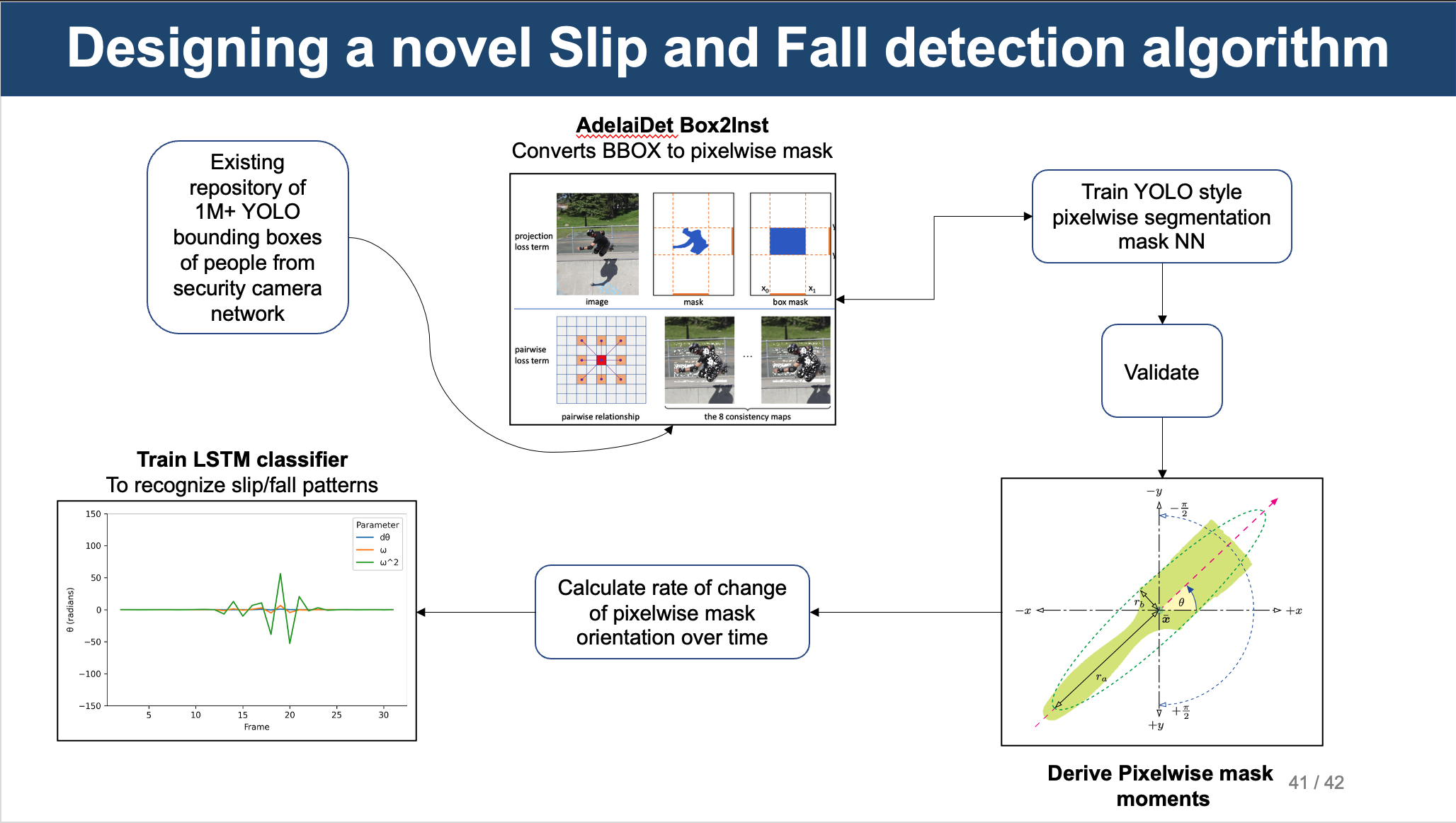
Furthermore, another caveat with working with security cameras is that in order to emphasize detection speed, it is favorable to use YOLO models. These usually require bounding boxes of people as training data. I had a ton of this data on hand while working at Actuate. As a prototype project, I thought I could use a bounding-box to pixelwise estimation model to grok the instance mask of a person. Then, using this data I further trained up a YOLACT model to track the person’s instance mask over time. Using mask moments I was able to calculate the principle axis of the mask approximated over a time window then train up a LSTM to classify if a person was standing or falling.
Learn why cancer grows the way it does
Lots of people today are pilled on either single-cell genomics or spatial transcriptomics. While these are either destructive or non-destructive ways to study cancer cells or cancer tissue in-situ they are not very powerful tools because cancer grows over space, and, crucially, time. If people do study cancer cells over time, they’re usually piecing a timeline of events from multiple populations of cancers across different patients and its usually met with mixed results each time.
The holy grail is to study the same cancer over time from the initial cell all the way to the final size it grows against (whether that’s when the patient is dead or when the cancer hits a boundary condition). Fortunately, I devised a way to study this (forthcoming blog post). What I can say is that when I did study it this way, I found out why cancer tissue grows in a similar pattern every time, even though no two cells are identical.
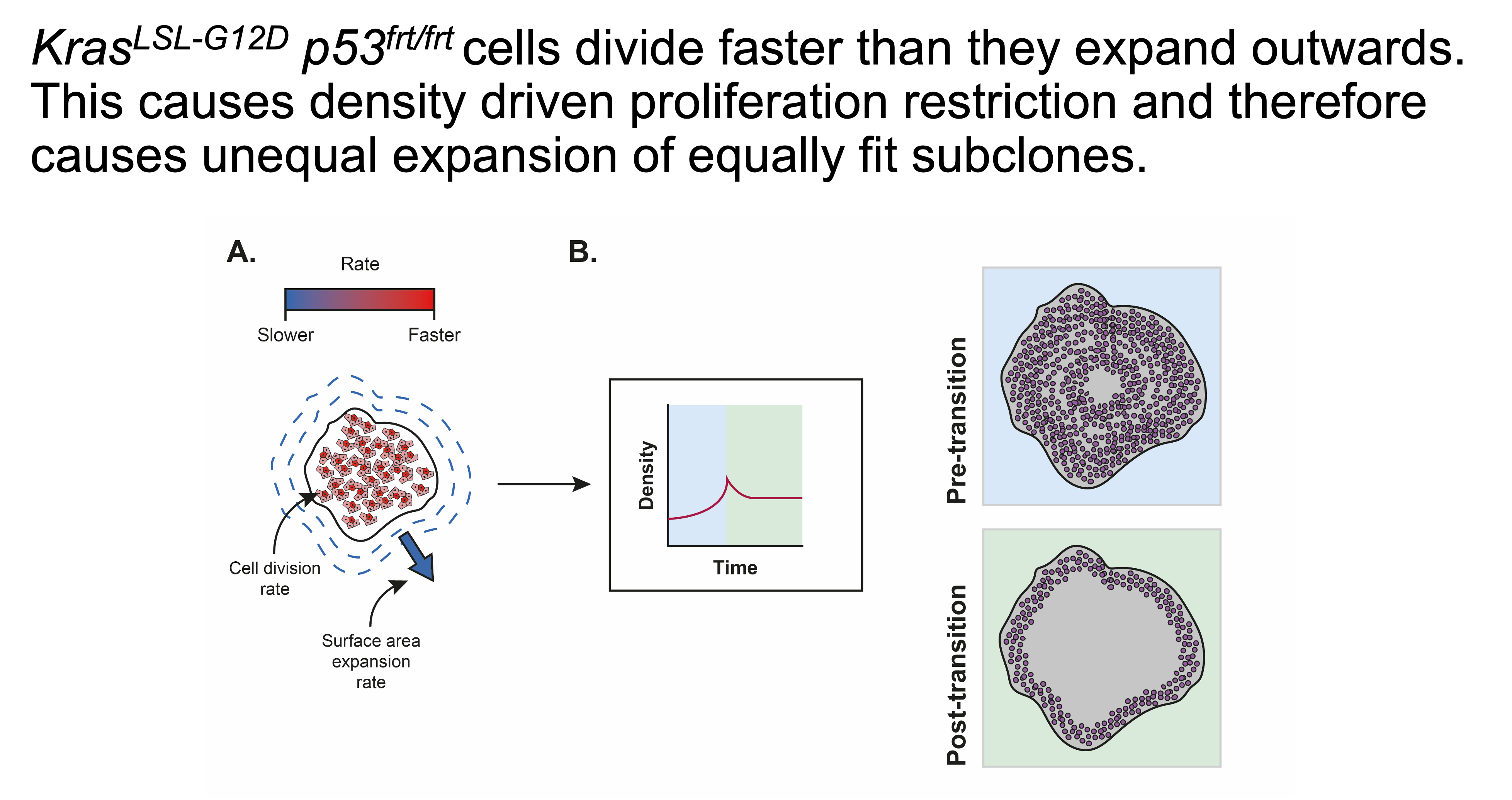
To create time-series data from imaging data is incredibly challenging and yet incredibly powerful because you can glean how each individual cell behaves within a crowded space over time. By leveraging the right analysis methods for spatiotemporal datasets, you can essentially study matter in the way it actually exists in our world.
Track exactly where your package was dropped off
Ok, now on to the subject of this post. I’ve been fascinated by the value proposition of Doorstep.ai. It appears from their website that they are a company that is interested in tracking the last 50ft of the delivery into your building. If you live in a major city and you don’t have a doorman in your building, you know exactly what this pain is.
According to a ChatGPT driven business estimation via web-search, U.S. carriers absorb roughly $16 billion in write-offs every year when parcels disappear inside buildings or get mis-scanned at the door. A 9-DoF sensor fusion SDK that runs on a driver’s phone to generate a verifiable indoor drop-point coordinate could cut “lost in the last 50 ft” claims by about 30 percent and turning those savings into measurable ROI.
Doorstep.ai’s SDK and data collection
Intriguingly they have a SDK that ostensibly runs on the delivery driver’s phone.
import React from 'react';
import { DoorstepAIRoot } from "@doorstepai/dropoff-sdk";
const App = () => (
  <DoorstepAIRoot apiKey="YOUR_API_KEY">
);
export default App;

// Injection of collection data via SDK
// Start with Google PlaceID
DoorstepAI.startDeliveryByPlaceID("placeID_here");

// Start with Google PlusCode
DoorstepAI.startDeliveryByPlusCode("plusCode_here");

// Start with Address Components
const address = {
    street_number: "123",
    route: "Main St",
    locality: "City",
    administrative_area_level_1: "State",
    postal_code: "12345"
};
DoorstepAI.startDeliveryByAddressType(address);
9-DoF sensor data
The basic premise of a 9-DoF sensor is that it can collect data from the following sensors:
| Sensor | Description |
|---|---|
| Accelerometer | 3-axis accelerometer |
| Gyroscope | 3-axis gyroscope |
| Magnetometer | 3-axis magnetometer |
| Light | Light sensor |
| Audio | Audio sensor |
| Barometer | Barometric pressure |
| GPS | Global Positioning System |
These chips are on the phone’s System on a Chip (SoC) but conceptually they are measuring the movement of a “ball” inside a box with sensor endings. Graphically, it looks like this:
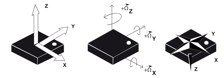
The 9-DoF sensor is a very powerful sensor that can be used to track the movement of a “ball” inside a box with sensor endings.
I sought out to figure out how to build a ML model that could carry out useful classifications on the data collected by this SDK.
Now, because I don’t have access to Doorstep.ai’s data, I had to find my own. Below and in the rest of the blog post, I yap about my casual 2-day journey to build a model and inference server that could run on the data collected by this SDK. Ostensibly by the end you will learn how I have deployed an inference server that could be passed the data collected by the SDK and be used to fill out a dropoff report that a customer could access if they have trouble locating the parcel in their building.
Finding phone sensor data
There are many datasets available. I ended up going for the ExtraSensory dataset because it did not require too much data cleaning and preparation to get started, though, the SHL dataset is very appealing.
| Dataset (year) | Core modalities present | Needs a “GPU”? | Inside/Outside labels? | Commentary |
|---|---|---|---|---|
| ExtraSensory (UC San Diego, 2017) | Acc, Gyr, Mag, Air pressure, Light, 22 kHz audio, phone-state, GPS, temp/humidity | 60 users ⇒ 302 k 20 s windows (≈22 h raw audio + high-freq motion; ~8 GB raw, ~215 MB features) (dcase-repo.github.io, kaggle.com, dcase-repo.github.io) | Yes (self-reported “indoors/outdoors” & “in vehicle”) (pmc.ncbi.nlm.nih.gov) | Full multimodal fusion + noisy labels + class imbalance |
| Sussex-Huawei Locomotion (SHL, 2018) | Acc, Gyr, Mag, Microphone audio, Baro, GPS, humidity, 15 total phone sensors (researchgate.net, eecs.qmul.ac.uk) | 2 812 h; 950 GB raw; 4 phones × 59 days preview (~20 GB) (shl-dataset.org, eecs.qmul.ac.uk) | Yes (explicit inside/outside tag) (eecs.qmul.ac.uk) | Scale & placement robustness; show distributed training |
| OutFin (Scientific Data, 2021) | Acc, Gyr, Mag, Baro, Light + Wi-Fi, BT, cellular (nature.com, nature.com) | 122 outdoor sites, dense fingerprints (~5 GB) (nature.com) | Outdoor-only (good negative set) | RF + sensor fusion for GNSS-denied environments |
| Opportunity++ (2021) | 72 sensors: body IMUs, object IMUs, ambient switches; video; no light, no audio (opportunity-project.eu, frontiersin.org) | 10 modalities, >4 GB raw time-series/video | Primarily indoor | Wearable + ambient devices; discuss aligning heterogeneous rates |
Preparing the data for a model
As you can probably imagine, most time-series datasets are not entirely the cleanest. They’re also so information dense that its hard to apply the entire dataset for a model. This section, therefore, talks about the Lets start with the basics of the ExtraSensory dataset.
- It is a dataset from 60 users.
- Participants were asked to install a companion app on their phone.
- Time sampling was every 20 seconds for every minute. Data is boxed by the minute on the dataset.
- Participants were given an easy method to report the state that they were in (walking, driving, indoors, outdoors, etc.)
Therefore, by definition the dataset is a multi-variate time-series dataset. Thinking about doorstep.ai’s value proposition of providing precise dropoff location accuracy, I decided to focus on whether or not one could identify whether or not the delivery driver was outdoors or indoors. Ostensibly, this is a binary classification problem.
Downloading the dataset
A full guide to how I download the dataset is in the repository here. I make extensive use of modal because I love their serverless GPU platform oh so much. I will gush over them throughout this blog post so if you’re a modal hater then you can stop reading now.
CREDENTIALS = modal.Secret.from_name(
    "aws-secret",
    environment_name="main",
    required_keys=[
        "AWS_ACCESS_KEY_ID",
        "AWS_SECRET_ACCESS_KEY",
    ]
)

app = modal.App(
    name="extrasensory-download",
    image=download_image,
)

@app.function(
    volumes={
        "/mnt": modal.CloudBucketMount(
            bucket_name=BUCKET_NAME,
            secret=CREDENTIALS,
        )
    },
    timeout=60 * 60 * 3,
)
def download_extrasensory_data():
    ...
Out of principle when I’m working with machine learning datasets I try not to have anything downloaded to my computer. This is because of potential data leakage and security concerns on top of the fact that these datasets are freaking massive and as such are not a good candidate to just hold in my computer at all times. Fortunately with modal I can just mount any old S3 bucket as a path and then use it as a local path. This is pretty convenient.
Discovering temporal windows
Intuition
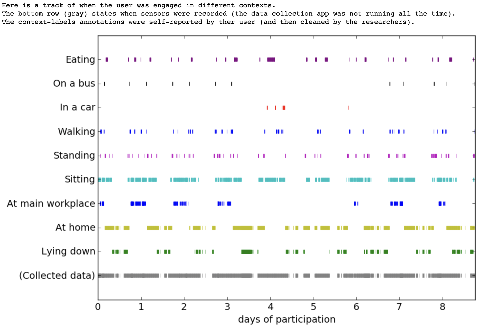
This dataset is a semi-continuous log of the phone’s sensors in multiple different contexts. If you were to just chuck all the data into a model, you’d likely have poor discrimination between the outdoor and indoor class because there are so many additional contexts that the person is in. For example a person can be outside but also inside a car. Indeed this is captured by the author and can be better described in the Youtube video linked to this dataset. Furthermore, this graph clearly articulates all the captured contexts for a typical user in the study.
Diving a bit deeper, the dataset contains temporal windows of the following phone sensors:
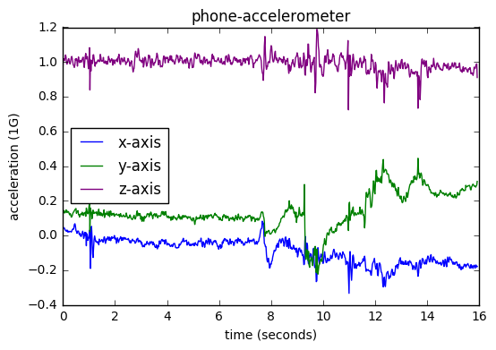
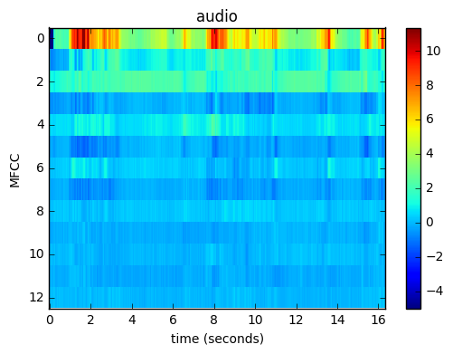
I had a thought. What if i narrow the context of the data to be used in the model to the point in the dataset where the person is transitioning between the outside and inside (e.g. immediately upon entering an enclosed building or leaving it?) This would increase the relevant number of samples to a value twice the number of users in the dataset.
\[N_{\text{after}} = 2\sum_{u=1}^{U} S_u = 2\,N_{\text{before}}\]The number of samples after the temporal window is narrowed is twice the number of samples before the temporal window is narrowed. Implementing this in python required a bit of work but ultimately resulted in the desired effect, I had more temporal windows to work with that narrowly described the transition between the outside and inside class within a specified window of window_size.
Implementation
def mark_transition_windows(X, col_inside, col_outside, window_size, label_names, new_label_names):
    """
    Mark transition windows in the data matrix X for transitions between two mutually exclusive labels.

    This function adds three new boolean columns to X:
        - The first new column is True for samples in a window before each transition.
        - The second new column is True for samples in a window after each transition.
        - The third new column is True at the exact transition point.
    The names for these new columns are provided by new_label_names and appended to label_names.

    Parameters
    ----------
    X : np.ndarray
        The input data matrix of shape (n_samples, n_features).
    col_inside : int
        The column index in X corresponding to the "inside" label (binary: 0 or 1).
    col_outside : int
        The column index in X corresponding to the "outside" label (binary: 0 or 1).
    window_size : int
        The number of samples before and after the transition to mark as the window.
    label_names : list of str
        The list of existing label/feature names (length should match X.shape[1]).
    new_label_names : list of str
        The list of 3 names for the new columns (e.g., ["left_window", "right_window", "transition"]).

    Returns
    -------
    X_new : np.ndarray
        The augmented data matrix with three additional boolean columns indicating:
            - Before transition window
            - After transition window
            - At transition point
    label_names_new : list of str
        The updated list of label/feature names with the new column names appended.

    Notes
    -----
    - Assumes that the "inside" and "outside" columns are mutually exclusive (never both 1).
    - Transitions are detected as changes in the "inside" label.
    - If a transition window would extend beyond the bounds of X, it is skipped.

    Example
    -------
    >>> X_aug, label_names_aug = mark_transition_windows(
    ...     X, col_inside=0, col_outside=1, window_size=5,
    ...     label_names=feature_names,
    ...     new_label_names=["left_window", "right_window", "transition"]
    ... )
    """
    n, old_cols = X.shape
    X_new = np.hstack([X, np.zeros((n, 3), dtype=bool)])
    inside = X[:, col_inside]
    outside = X[:, col_outside]
    assert np.all((inside + outside) <= 1), "Labels must be mutually exclusive"
    inside_diff = np.diff(inside.astype(int), prepend=inside[0])
    transitions = np.where(inside_diff != 0)[0]
    for idx in transitions:
        start = idx - window_size
        end = idx + window_size + 1
        if start < 0 or end > n:
            continue
        X_new[start:idx, old_cols] = True         # Before
        X_new[idx+1:end, old_cols+1] = True       # After
        X_new[idx, old_cols+2] = True             # At transition
    label_names_new = list(label_names) + list(new_label_names)
    return X_new, label_names_new
Visual Description
Visually this could also be described as the graph below. The transition points are marked in purple with the before and after window of ~5 minutes marked in red and green respectively. The analysis isn’t completely perfect but it is directionally correct for the length of time I worked on this for a proof of concept.

Cleaning and preparing the dataset
I then ran a clean of the potential np.nan and np.inf values that would most defintiely interfere with a multi-variate classification model. This can be found in the github repository here. Running the code below resulted in a labels array that described the classes of the data. The final shape of the labels array was (4293,). The final shape of the dataset was (4293, 5, 225)
# Inside is 0, Outside is 1
labels = np.concatenate(
    [np.zeros(len(inside_windows), dtype=int),
    np.ones(len(outside_windows), dtype=int)]
)
Building the model
Its my belief that unless you’re writing a machine learning model from scratch (which you’re probably not going to be doing if you’re supporting most business cases) you’re going to be using a library to build your model. This has caveats. The caveats being that you’re beholden to the library’s design choices and support requirements to deploy your model. That being said, there are some pretty robust model libraries out there, and tsai is no exception. Training with tsai is easy because it is built ontop of fastai. Because of this, and recent developements to the TSClassifier class, deploying a model is as simple as running the code below. I will note there are a few caveats and these will be discussed.
The tsai library
Configuring a TSClassifier requires a dictionary with some typical parameters in any machine learning job:
# Configruation Dictionary
config = {
    "tfms": [None, TSClassification],
    "batch_tfms": [TSStandardize(by_sample=True)],
    "metrics": accuracy,
    "arch": "InceptionTimePlus",
    "bs": [64,128],
    "lr": 1e-4,
    "epochs": 5,
}
I chose to split my data into test and train at the point of the model training. I prefer to keep my data as tight as possible to the model training process.
train_index, val_index = train_test_split(np.arange(len(dataset)), test_size=0.2, random_state=42, stratify=labels)

# Splits
splits = (list(train_index), list(val_index))
Then finally training the library is as simple as running the code below.
# Create Model
learn = TSClassifier(
    X=dataset,
    y=labels,
    splits=splits,
    tfms=config["tfms"],
    batch_tfms=config["batch_tfms"],
    metrics=config["metrics"],
    arch=config["arch"],
    bs=config["bs"],
    cbs=[WandbCallback(log_preds=False, log_model=False, dataset_name="extrasensory-train")],
)

# Train Model
learn.fit_one_cycle(config["epochs"], config["lr"])
InceptionTimePlus Intuition
I was at UofT doing my Masters in Biochemistry around the same time that Ilya Sutskever was working on the original AlexNet. There is a lot of influence from the original AlexNet in my own understanding of NN architectures and my background and interest in computer vision partly stems from this. I was therefore excited to use InceptionTimePlus as a model architecture for this project. Indeed the paper does pay quite a bit of homage to the original AlexNet when drawing parallels between the two model architectures.
There are many ways to classify time-series data. Most of the approaches are interested in finding features (shapelets, spare-representations, etc.,) that are invariant to the time-index of the time-series.
-
Nearest Neighbor + NN-DTW: The NN-DTW approach is well described in this blog post.
-
BOSS: Breaks the time-series into symbolic features via discrete fourier transform. Then discretizes the features into bins, and if I’m getting this right, measures the euclidean distance between the features.
InceptionTime works in a similar way as AlexNet. You have a sliding window of m filters on the multivariate time-series. In the case of my dataset its 225 features over 5 minutes. What this does is that it reduces the dimensionality of the time-series from 225 features to the number of filters. This “bottlenecking” reduces the multi-variate features of the feature space (that’s accelerometer, gyroscope etc.,) to a set of m filters.
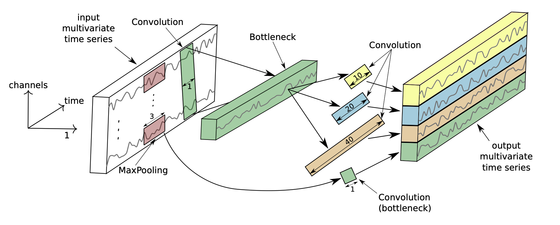
You can think of this the same way as a multi-dimensional image. If you’ve ever worked in science and have used the .czi format from Zeiss you know that a typical fluorescence image can be a 4-30 dimensional image based on the number of channels collected at various filter-band passes or excitations based on your laser. Time series works the same way in the multi-variate space. The time dimension is only collapsed in the very last layer. What happens there is just some pooling of the time-series against the collapsed m features from the sliding window over the time-series. This is also why making sure you choose a temporal window that’s cleanly defined is so important.
There are obviously different are more interesting filters one could conjure up for time-series data but this method is a good starting point and a good model architecture.
Weights and Biases Callbacks
You’re probably wondering what is this WandbCallback? Its a fastai callback that logs the training and validation metrics to Weights and Biases. I’ve found this to be a very useful tool for tracking the training of my models.
# Create Model
with wandb.init(project="extrasensory-train", name="extrasensory-train"):
    learn = TSClassifier(
        cbs=[WandbCallback(log_preds=False, log_model=False, dataset_name="extrasensory-train")],
    )
Tracking training runs and validation metrics is then possible on wandb.ai which you can find here.
Running inference on using the model
Running inference (owing to the amazing work of the tsai library) is as simple as running the code below.
@app.cls(
    image=inference_image,
    gpu="any",
    scaledown_window=60 * 10,
    volumes={"/weights": weights_volume},
)
class Inference:
    @modal.enter()
    def start(self):
        wandb.init(mode="disabled")
        self.model = load_learner(f"/weights/{MODEL_ID}", cpu=False)

    @modal.method()
    async def predict(self, data: np.ndarray):
        return self.model.get_X_preds(data, with_input=False)
You can call this from an ASGI remotely as follows:
####
# Request Model
####

class Request(BaseModel):
    array: str

class Result(BaseModel):
    probabilities: list
    predicted_class: str
    message: str

####
# ASGI Application
####

@app.function(
    image=asgi_image,
    max_containers=2
)
@modal.asgi_app(label="extrasensory-inference")
def extrasensory_inference():
    application = FastAPI(title="Extrasensory Inference", description="Inference for the Extrasensory Model")

    # Inference endpoint
    @application.post("/predict", response_model=Result)
    async def predict(request: Request = Body()):

        bytes = base64.b64decode(request.array)
        array = np.load(io.BytesIO(bytes))

        if array.shape != (1, 5, 225):
            return {"error": "Invalid array shape"}

        # Make prediction - don't await the remote call
        response = Inference().predict.remote(array) # type: ignore

        # Unpack the tuple and convert tensor to numpy
        probs_tensor, _, class_label = response
        probabilities = probs_tensor.cpu().numpy().tolist()
        predicted_class = class_label[0]

        return Result(
            probabilities=probabilities,
            predicted_class=predicted_class,
            message="Success"
        )

    return application
It will return a JSON object with the probabilities of the predicted class and the predicted class label.
{
    "probabilities": [0.9999999403953552, 4.964479923248291e-07],
    "predicted_class": "outside",
    "message": "Success"
}
Caveats
wandb Callbacks
One very peculiar thing I noticed and spent a needless amount of time on was the need to have the wandb callback or at least the wandb library instantiated before the prediction model was instantiated. I thought it was weird that the pickled model required the wandb library. This might’ve been due to the fact that one of the model callbacks was a wandb callback.
wandb.init(mode="disabled")
Sparsity of the dataset
The Extrasensory dataset was sampled at a rate of 1 minute. Events such as walking between inside and outside happen at a much faster frequency than 1 minute. This means that the model and its ability to generalize for indoor versus outdoor classification might be limited. Ideally you’d want a sampling frequency of at least once per second or even faster. This would pose challenges from a battery life perspective and potentially pose challenges if the data was uploaded to the cloud when the phone is in wifi range.
Gushing over Modal
Its no secret that I gush over Modal. I particularly liked the ability to use modal.CloudBucketMount to mount a S3 bucket as a local path and then a modal.Volume to mount a volume to the container. Container definition on Modal is just so dead simple. Defining infrastructure should be this easy:
@app.function(
    volumes={
        "/mnt/": modal.CloudBucketMount(
            bucket_name=BUCKET_NAME,
            secret=CREDENTIALS
        ),
        "/weights": weights,
    },
    timeout=60 * 60 * 3,
    secrets=[WANDB_SECRET],
    gpu="any"
)
Some of my next learnings are going to be how to chain all these files together into a single pipeline. It would be cool to just run one script to download the data, train the model, and deploy the model.
Conclusion
Even though I didn’t get the job at Doorstep.ai, I am happy to have had the opportunity to work on this project. I really love working on time-series data and I’m excited for others to take note of the codebase for their own projects.